I was working on an excel sheet with over 10,000 values in which there were multiple duplicates, triplicates and used this method to help me sort the duplicates/triplicates.
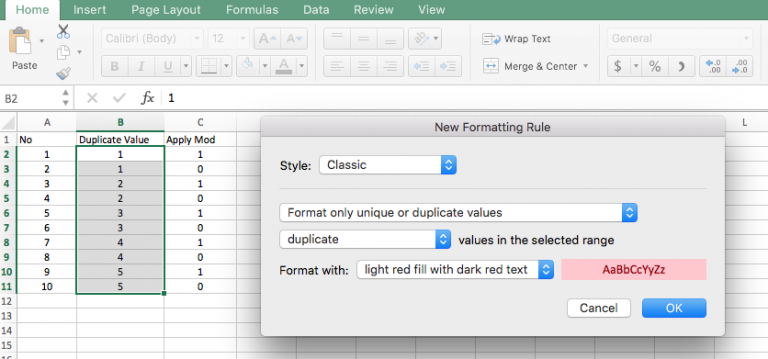
The first thing was to do is to select the entire column and select duplicates as show in fig 1

fig 1
Click on duplicates as in fig 2
fig 2
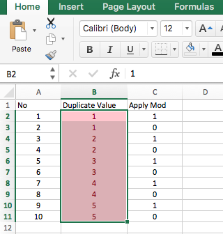
After you click on “OK” all the duplicate values will appear as in fig 3
fig 3
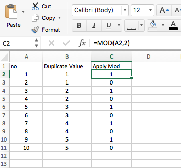
Then in the “Apply Mod” as in fig 4 use the forumla =mod(A2,2) where “A2” is the column/row name and “2” is the number of duplicate values. In this case for each value there is a duplicate and if for each value there is a triplicate then use “3” instead of “2”. Then populate the entire column with the calc by dragging it down or double clicking it in the corner of the cell.
fig 4
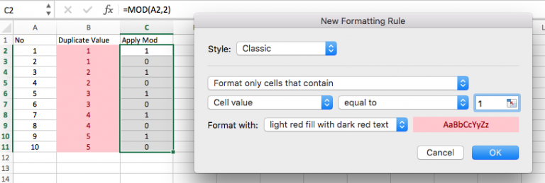
Select column “Apply Mod”, then from fig 1: Select conditional formating -> Highlight cell rules -> Equal to as in fig 5. In the “Equal to” value enter “1′ or “0”
fig 5
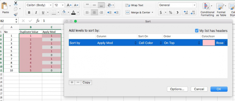
If you enter ‘1’ in fig 5 then all ‘1’ will be a rose color like ‘Duplicate value’. Then sort the cell color under ‘Apply Mod’ as shown in fig 6
fig 6
When you click ‘ok’ the rose colored cells in the ‘apply mod’ will be on top. You have now separated the duplicates.
Do let me know how this helped you in the comments.
